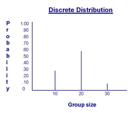
Discrete Distributions

Building the Model: Advanced Elements > User Defined Distributions > Discrete Distributions

Discrete Distributions

Discrete distributions are characterized by a finite set of outcomes, together with the probability of obtaining each outcome. In the following example, there are three possible outcomes for the group size: 30% of the time the group size will be 10, 60% of the time the group size will be 20, and 10% of the time the group size will be 30.

One way to represent a discrete distribution is by its probability mass function, listing the possible outcomes together with the probability of observing each outcome. A probability mass function for the example above could be expressed as follows (with G representing the group size).

G 10 20 30

P(G) .30 .60 .10

An alternate way to represent a distribution is through a cumulative distribution function, listing each possible outcome together with the probability that the observed outcome will be less than or equal to the specified outcome. A cumulative distribution function for the example above could be expressed as follows.

G 10 20 30

P(G) .30 .90 1.0

In the next example, the number of parts are grouped into a batch according to a user distribution.

Process Table

Entity...	Location...	Operation (min)...
EntA	Loc1	GROUP Dist() AS Batch
Batch	Loc1	WAIT 10 min

Routing Table

	Output...	Destination...	Rule...	Move Logic...

1	Batch	Loc2	FIRST 1	MOVE FOR 5

MedModel provides the flexibility to specify discrete distributions according to a probability mass function or a cumulative distribution function. Select Yes or No in the Cumulative field of the Distribution edit table and fill in the table according to the probability mass function or the cumulative distribution function. The following tables show the discrete distribution example defined in both formats.

Discrete Distributions

Discrete (probability mass function)

Discrete (cumulative distribution function)